Engineering overview
Senstar OmniTrax concealed perimeter system: operating principle and architecture
A look inside the design and operating principle of Senstar OmniTrax: how the detection zone is formed, which components make up the system, how the perimeter is divided into alarm zones, how the system is calibrated on site, and how to size the kit for a boundary of a given length.
Fence-mounted sensors, microwave barriers, and thermal cameras all have one thing in common: they are visible. An intruder can see where the detection boundary is, assess its location, and plan how to bypass it. A buried cable detection system works differently. The detection boundary exists — but there is nothing visible on the surface.
Solution Class and Its Role in the Security Architecture
OmniTrax belongs to the class of leaky coaxial cable detection systems — a buried RF sensor technology based on perforated, or ported, coaxial cable.
Within a layered perimeter security architecture, OmniTrax serves as a detection layer — not a physical barrier. It does not stop an intruder or replace a fence. Instead, it detects a perimeter breach, determines its location, and reports the event to the higher-level security system. From there, video surveillance, security lighting, and response personnel take over.
The system is typically deployed in one of two roles.
As a standalone concealed detection layer — for sites where visible perimeter protection is not an option, including prestigious properties, heritage sites, and facilities where the security boundary should remain invisible.
As an inner detection layer behind a visible fence — an intruder who has crossed the perimeter fence remains unaware of the second detection layer and is unlikely to anticipate it. This is a classic defense-in-depth architecture widely used to protect critical infrastructure.
The technology is typically most cost-effective for perimeters ranging from approximately 200 meters to several kilometers. On shorter perimeters, the fixed cost of the controller and system commissioning is spread over too little protected distance, making the overall solution less economical.
Operating Principle
How the Detection Zone Is Formed
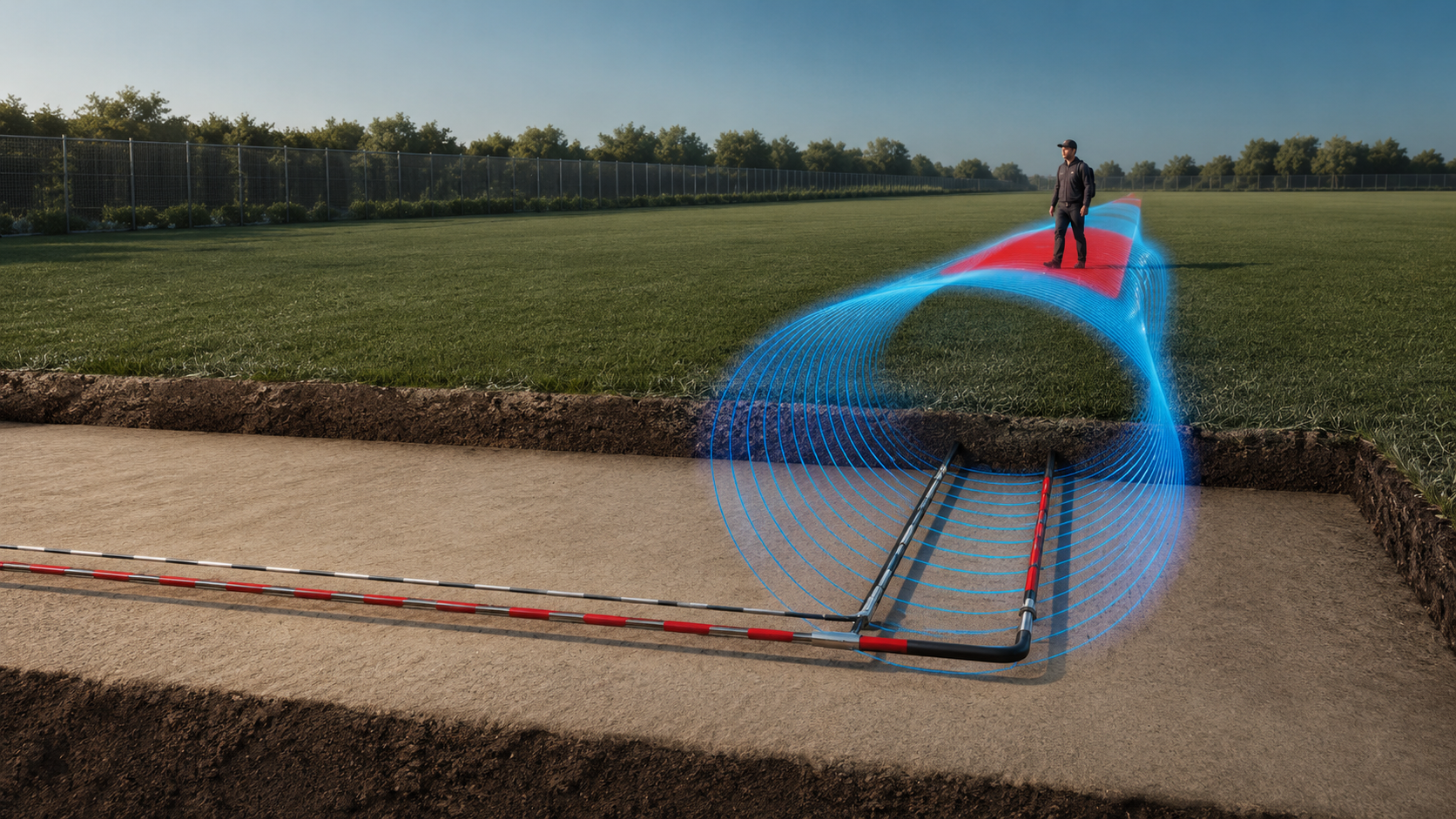
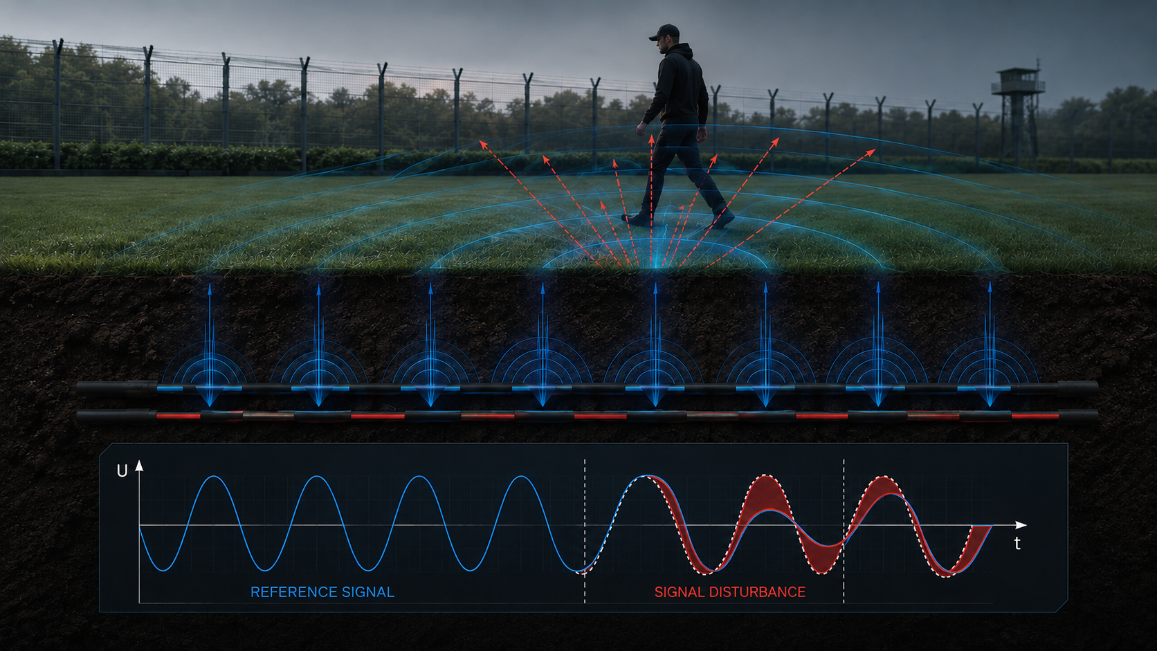
The sensing element consists of two parallel coaxial cables buried in the ground.
The transmitting cable has a perforated outer conductor — hence the name ported, and, from the character of its operation, leaky. Because the shielding is intentionally incomplete, a portion of the RF energy radiates into the surrounding ground. A parallel receiving cable captures this energy. The system operates at a carrier frequency of 32.125 MHz.
Under normal conditions, a stable RF field is established between the two cables. When a person enters the detection zone, their body reflects and disturbs the electromagnetic field. The receiver detects these changes, which serve as the signature of an intrusion.
What the Controller Analyzes
The controller processes the received signal in four stages.
Amplitude analysis
Signal amplitude is proportional to the target’s size, which yields an estimate of the object’s dimensions.
Phase analysis
Detects object movement within the detection zone.
Signal duration analysis
Yields the object’s speed.
Correlation of all characteristics over time
The critical stage, and the one that filters out environmental disturbance: an alarm is generated only when the expected target characteristics — object size, movement, and speed — are all detected within the same time window.
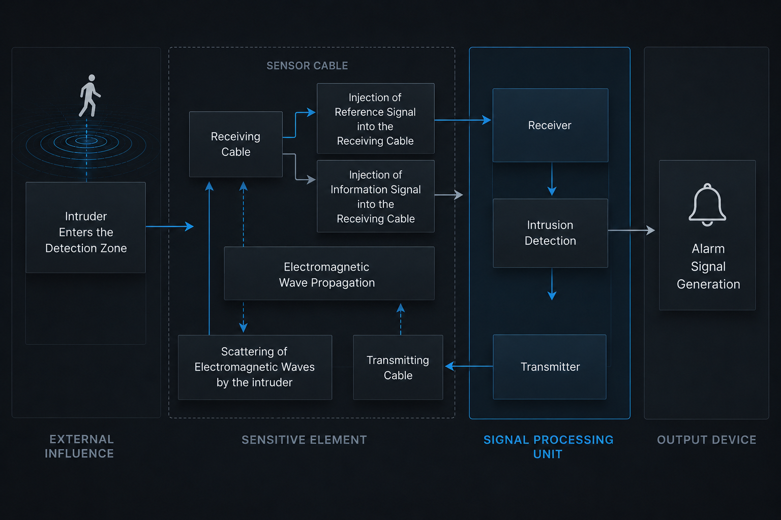
This signal processing approach explains the system’s immunity to environmental influences such as wind, rain, snow, hail, sandstorms, fog, extreme temperatures, seismic vibration, acoustic noise, and magnetic interference. While these conditions may disturb the electromagnetic field, none produces the combination of target size, movement, and speed required to generate an alarm within the same observation window. For the same reason, moving vegetation — including grass, shrubs, and trees — does not trigger alarms.
Sensor Operating Window
Probability of detection (Pd) — over 99% at a 95% confidence level. Conditions: target weight over 35 kg, upright orientation, target speed from 5 cm/s to 8 m/s. Objects weighing less than 10 kg are ignored — at the same 95% confidence level.
The speed range deserves a closer look: the upper limit of 8 m/s covers a running intruder, while the lower limit of 5 cm/s accounts for a slow, deliberate crossing. Both extremes remain within the sensor’s operating window.
Intrusion Localization
The system provides range-based intrusion localization. The controller analyzes the signal response across up to 40 range cells for each cable. By evaluating the signal amplitude and propagation delay within these cells, it determines the location of the intrusion. Position accuracy is ±1 m, with a possible deviation of up to 4 m due to phase ambiguity. The capability is based on patented coded-pulse signaling technology.
Coded-pulse signaling allows the system to localize multiple simultaneous intrusion attempts. The 24 m target separation resolution defines the limit of this capability: if two targets cross the detection boundary less than 24 meters apart within a three-second interval, the system will report them as a single intrusion event.
Precise location data is what fundamentally distinguishes OmniTrax from zone-based sensors. A PTZ camera can be directed to a specific point rather than a broad sector, and the operator sees the intrusion location on the site map rather than simply receiving an alarm from a section of the perimeter. When defining camera presets, the field of view should include sufficient margin to account for a possible deviation of up to 4 m — this ensures the target remains within the frame under any expected localization scenario.
Detection Zone Geometry
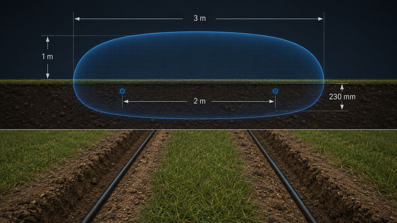
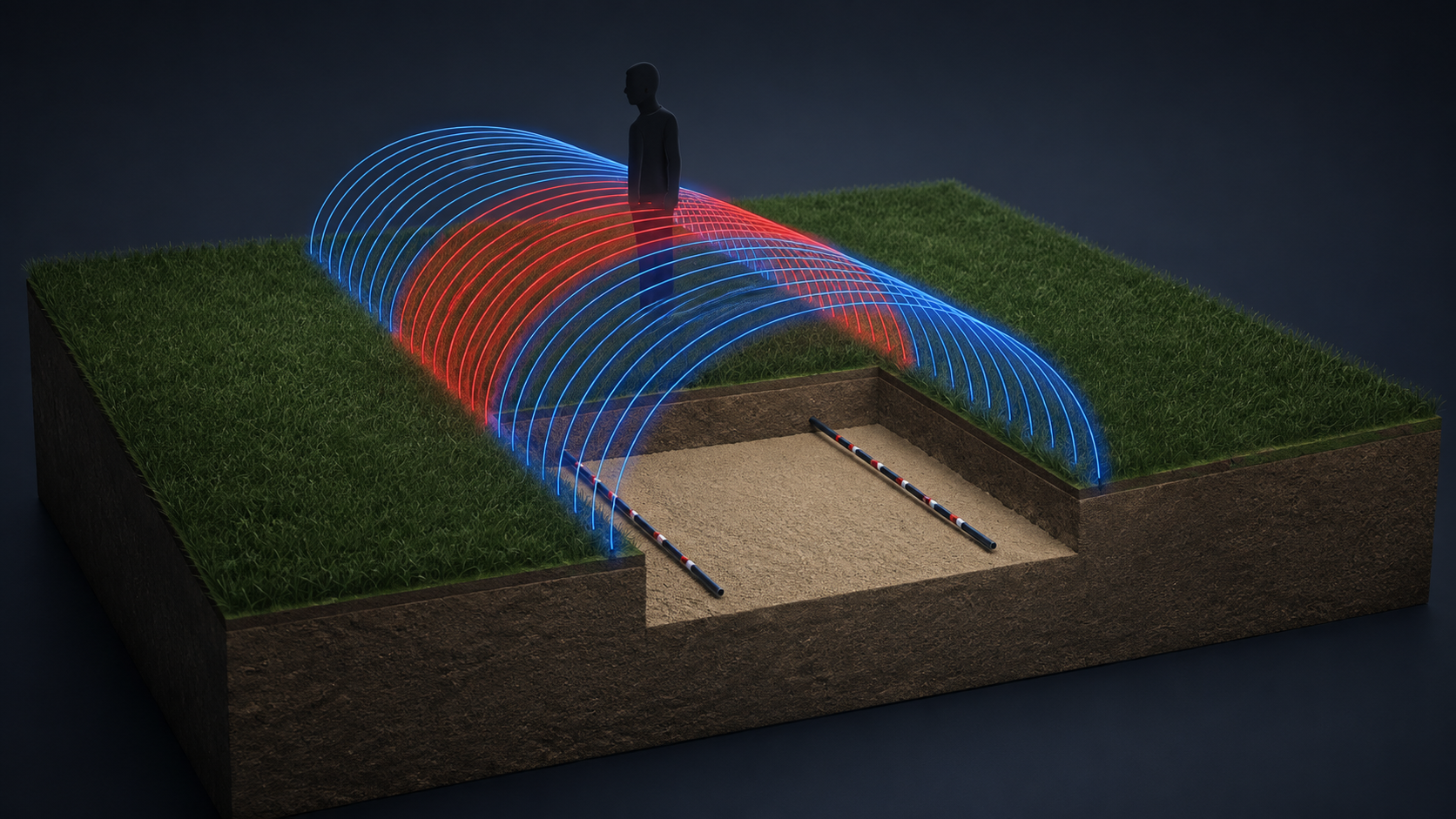
The detection zone has the shape of an elliptical cylinder. Its upper half extends above ground level, while the lower half lies below the surface. The cylinder’s longitudinal axis runs parallel to the cable route.
- Detection zone height — 1 m; width — 2–3 m, depending on cable spacing and site conditions.
- Minimum cable route bend radius — 7 m, measured along the centerline.
- A 90° turn through concrete openings — three consecutive 30° bends with a minimum spacing of 3.6 m.
- Maximum change in surface slope along the cable route — 30° over a 4 m distance.
The dimensions of the detection zone depend on the cable burial depth, the surrounding medium, the spacing between the cables, and the configured sensitivity threshold. The maximum width of approximately 3 m is achieved with the maximum cable spacing of 2 m; with the recommended spacing of 1.5 m, the detection zone is correspondingly narrower. For preliminary coverage calculations, the lower end of the width range should be used, with the actual detection zone verified and calibrated on site during commissioning.
The detection zone follows the terrain. This is a fundamental difference from microwave and optical beam sensors, which require a clear line of sight. Changes in elevation, slopes, and uneven ground are accommodated naturally — the detection boundary follows the cable route.
Cable Burial Depth
| Medium | Depth |
|---|---|
| Soil, sand–soil mixture, or gravel | 23 cm ± 2.5 cm |
| Medium to heavy clay | 15 cm ± 1.3 cm |
| Asphalt, large paved areas such as parking lots or runways | 23 cm ± 2.5 cm |
| Narrow asphalt strip (e.g. a driveway) with adjacent soil at 23 cm | 30 cm ± 2.5 cm |
| Unreinforced concrete, less than 13 cm thick | 23 cm ± 2.5 cm, trench cut and surface restored |
| Unreinforced concrete, more than 13 cm thick | 6 cm ± 6 mm saw cut |
| Reinforced concrete, any thickness | 6 cm ± 6 mm saw cut, with the cable installed at least 2.5 cm above the reinforcing steel |
Cable Spacing
The recommended spacing is 1.5 m, the minimum 10 cm, the maximum 2 m. The recommended 1.5 m should be used wherever site conditions allow: it provides the best signal-to-noise ratio and the widest, most uniform detection zone.
A cable spacing of 10 cm is also a fully supported installation configuration and offers a practical cost advantage: both cables can be installed in a single trench, significantly reducing excavation work. This is the most common approach where the available installation corridor is narrow.
The trench trade-off
A spacing of 1.5 m gives the widest uniform detection zone and the best signal-to-noise ratio. A spacing of 10 cm puts both cables in one trench — at the cost of a narrower detection zone and a lower signal-to-noise margin. The choice between 1.5 m and 10 cm depends on the available installation space and the project’s excavation budget.
System Components
Controller
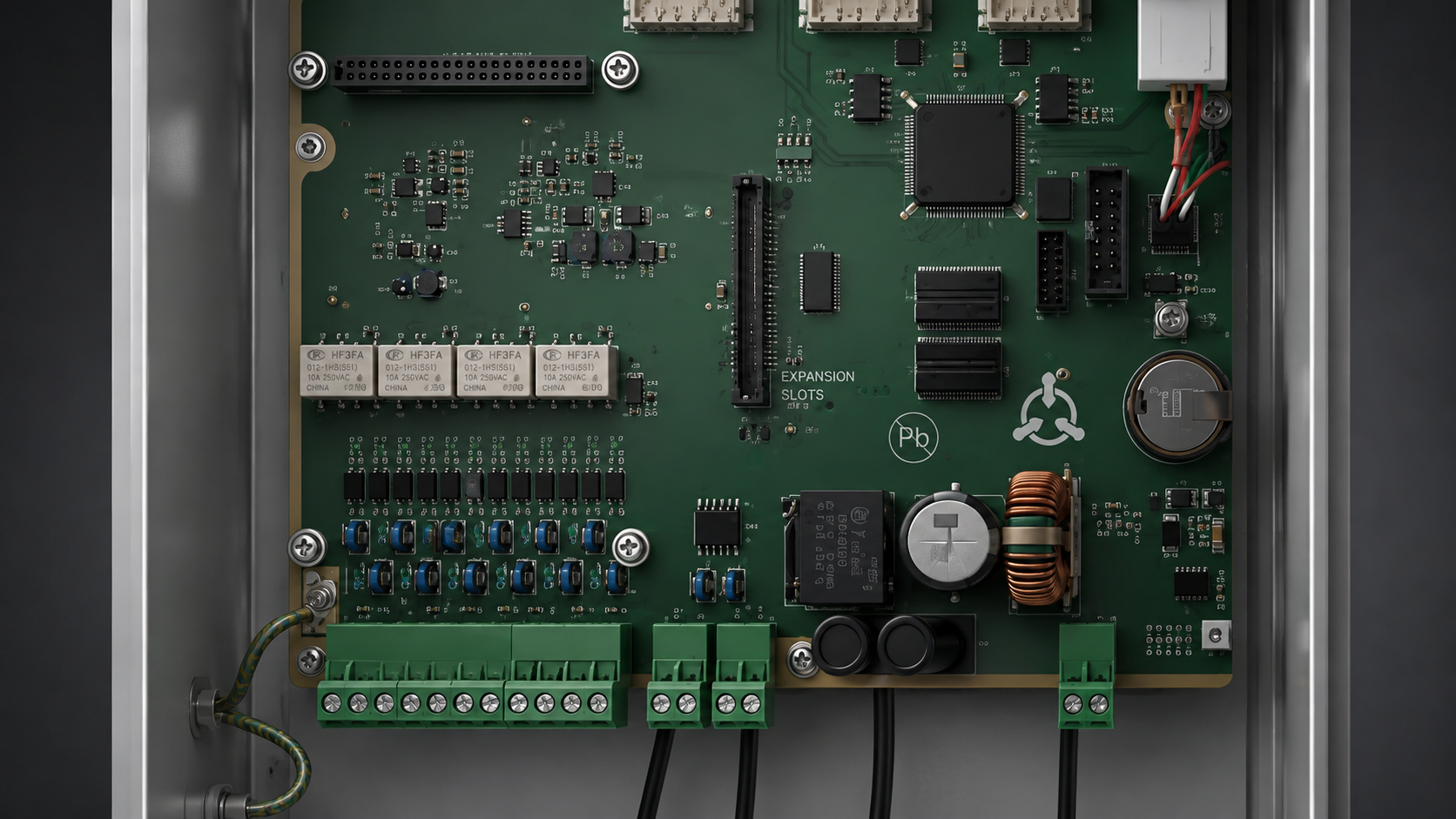
The controller is the core of the system. A single controller supports two sensor cable runs.
| Specification | Value |
|---|---|
| Maximum protected perimeter | Up to 800 m (two cable runs of up to 400 m each) |
| Enclosure | Painted aluminum, CSA/UL Type 4X |
| Dimensions (H × W × D) | 40 × 23.5 × 16.5 cm |
| Weight | 4.9 kg without battery |
| Power input | 12–48 VDC |
| Power consumption | Less than 9 W |
| Operating temperature | −40 to +70 °C |
| Relative humidity | Up to 95%, non-condensing |
| Sensor cable connections | Four TNC female (TNC-F) connectors |
| Cable entries | Four, with compression cable glands |
| Grounding | 5 Ω or less recommended |
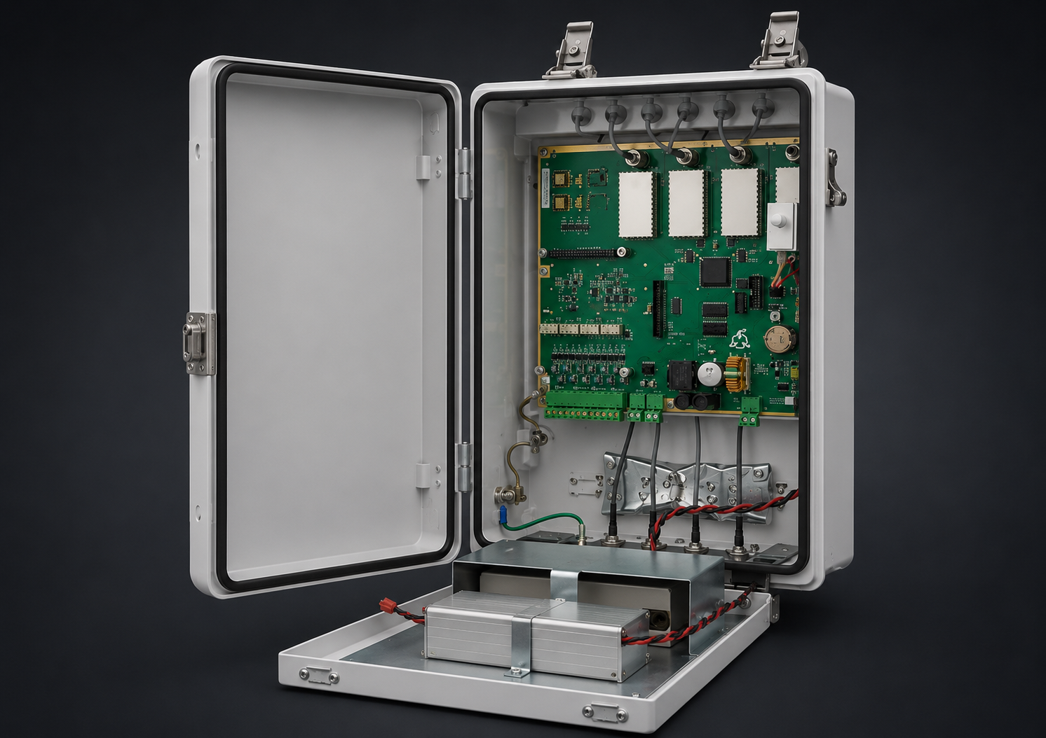
Backup power. The controller can be supplied with a backup battery, installed inside the enclosure on the door. In the base part number A4EM0101 the battery ships together with the controller; the 4.9 kg weight given in the table above is stated without it.
Backup power here is exactly that — backup: the battery is intended for emergency ride-through, not for the role of a primary source. On sites with an unstable mains supply, the issue is addressed with an uninterruptible power supply at the input. Capacity and autonomy time for a specific configuration should be agreed when placing the order.
Surge protection is built in: non-radioactive gas-discharge devices and transient-voltage suppressors protect all input/output ports, including relay outputs, communication lines, auxiliary device inputs, power inputs, and sensor cable connections.
Outdoor enclosure (optional) — designed for above-ground installation of the controller: 98.4 × 42.5 × 27.3 cm, steel with a light green enamel finish, rated IP33. A pole-mounting bracket is also available.
Sensor Cables
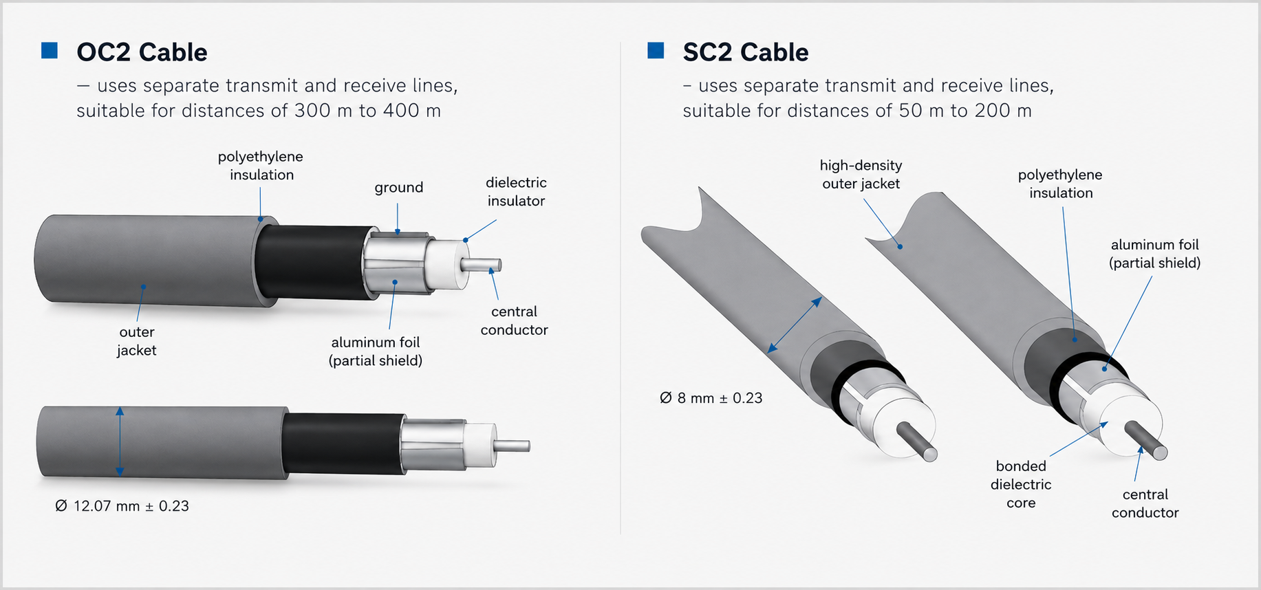
| Specification | OC2 | SC2 |
|---|---|---|
| Configuration | Separate transmit and receive cables | Separate transmit and receive cables |
| Available sensor cable lengths | 300 m, 400 m | 50, 100, 150, 200 m |
| Outside diameter | 12.07 mm ± 0.23 | 8.00 mm ± 0.23 |
| Lead-in cable length (non-sensitive) | 20 m | 20 m |
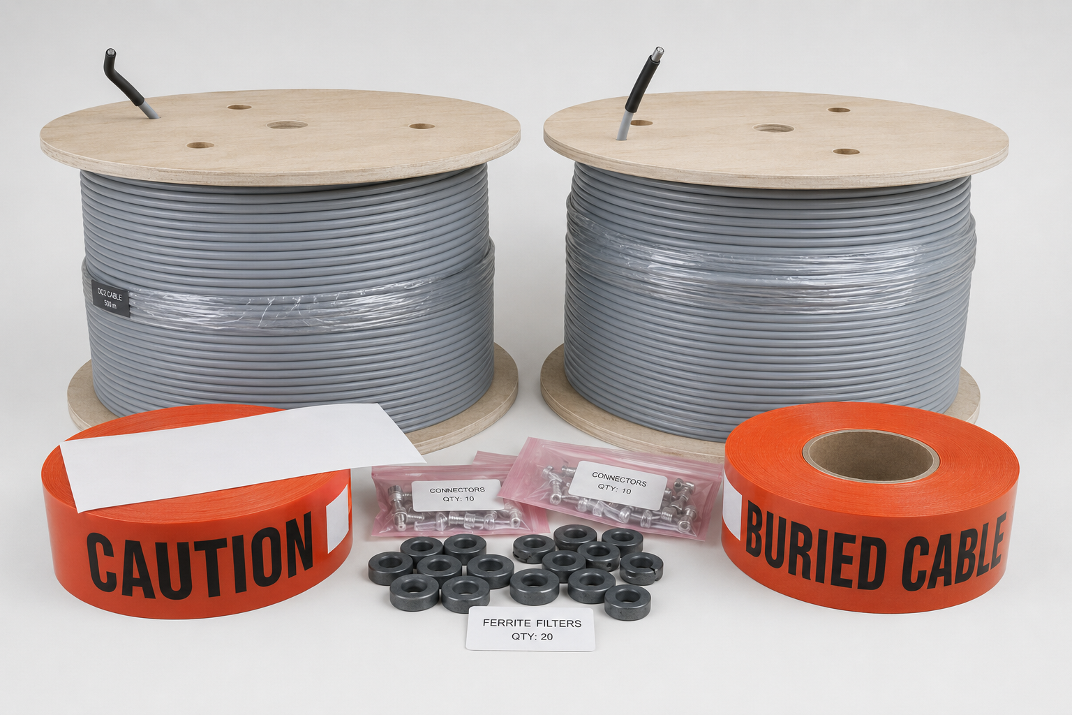
| TNC connectors included | 6 | 4 |
| Ferrite filters included | 42 | 20 — technical specifications table lists 10, see note |
| Marker tape | Three rolls of 305 m | Two rolls of 305 m |
| Maximum protected perimeter per controller | 800 m | 400 m |
| Typical applications | Long perimeters, cable-plow installation | Short perimeters |
Documentation discrepancy. Regarding the SC2 ferrite filters: the packing list specifies 20 filters, while the technical specifications table lists 10. Both figures are stated here deliberately; the actual quantity should be confirmed when placing the order.
Both cable types feature a graded cable design: the perforation size in the outer conductor varies along the length of the cable to compensate for signal attenuation. As a result, detection sensitivity remains uniform over the entire sensor cable length rather than decreasing toward the end of the cable run.
The non-sensitive lead-in section is a 20 m length of fully shielded cable that connects the controller to the start of the detection zone. No detection field is generated along this section, allowing the controller to be installed at a convenient distance from the protected perimeter. The transition between the lead-in cable and the sensitive section is identified by red bands.
Couplers and End-of-Line Terminations
Sensor cable assemblies are interconnected using couplers. A network coupler (with power pass-through) passes both data and DC power, and is used when DC power is distributed over the sensor cable. An isolated coupler (power-blocking) passes data while blocking DC power, and is used when each controller has its own local power supply.
End-of-line terminations are installed at both ends of an open-ended perimeter. They provide the electrical termination for both the detection zone and the data communication path.
Expansion Modules
The controller accepts one communication module and one I/O module.
The communication module handles communication between controllers, and its type sets the maximum distance: RS-422 over copper — up to 1.2 km, multimode fiber 820 nm — up to 2.2 km, single-mode fiber 1310 nm — up to 10 km.
The I/O module comes in two versions: a relay output module (8 Form C relays, 1 A @ 30 VDC) or a universal input module (8 supervised inputs with programmable thresholds). They are mutually exclusive: only one of the two can be installed at a time.
Built-in I/O
As standard, the controller provides 4 relay outputs (Form C, 1 A @ 30 VDC, resistive load) and 2 dry-contact inputs — one input per sensor cable run.
Each relay can be configured independently. In standalone operation, available relay assignments include alarm, supervision, enclosure tamper, power failure, and fault. Relay activation time is programmable from 0.125 to 10 seconds.
In standalone operation the dry-contact inputs are used for self-test functions; in networked operation they serve as auxiliary alarm inputs and can be configured for normally open or normally closed operation, with optional end-of-line resistor supervision.
Power Supply and Accessories
- 48 V, 100 W outdoor power supply — centralized power supply for multiple controllers.
- 12 V, 80 W local power supply — power supply for a single controller.
- Surge protection kit — external surge protection for sensor cables; one kit protects two sensor cable pairs connected to a single controller.
- Cable termination kits — tools and components for cable preparation and TNC connector termination; separate kits for OC2 and SC2 cables.
- Cable repair kits — repair of damaged cable sections.
From Meter-Level Localization to Alarm Zones
The system uses a three-level localization hierarchy.
Meter
The fundamental unit of localization. The sensitivity profile is recorded and calibrated independently for each meter of sensor cable.
Segment
A contiguous group of meters defined in software: configurable from one meter up to the full length of the sensor cable.
Alarm zone
One or more segments grouped together. The alarm zone is the level presented to the operator and used to drive the system response.
The limits are as follows: up to 50 segments per sensor cable assembly, up to 100 segments per controller, up to 50 alarm zones per controller, and a minimum segment length of 1 m.
The zoning model is more flexible than it may first appear:
- segments assigned to the same alarm zone do not have to be contiguous — a single zone can span multiple separated sections;
- zone length is independent of cable length — a 5 m zone can be defined around a gate while a 200 m zone covers a straight perimeter section;
- an alarm zone can contain another alarm zone;
- an alarm zone can span corners and skip inactive sections of the perimeter;
- a dedicated Zone 0 is reserved for the lead-in section and other inactive cable segments; it does not report target detections and is not counted toward the 50-zone limit.
There is one hard constraint: an alarm zone cannot span multiple controllers — a zone may include segments from both sensor cable runs connected to the same controller, but not segments assigned to different controllers. On multi-controller installations, this constraint determines where alarm zone boundaries must be placed.
In practice, this means the perimeter can be partitioned logically to match the video surveillance layout, response sectors, or areas with different threat levels — without relocating a single sensor cable. A high-traffic gate, for example, can be assigned to its own alarm zone with dedicated sensitivity settings, while the remainder of the perimeter continues to operate unchanged.
Power and Data over the Sensor Cable
This is the system’s primary infrastructure advantage. The sensor cable already installed along the perimeter serves three functions simultaneously: it forms the detection zone, distributes 48 VDC power to the next controller, and carries network communications.
In practical terms, this eliminates the need for separate trenching — one route for a power cable and another for a communications cable. On multi-kilometer perimeters, avoiding these additional cable runs can significantly reduce the amount of excavation required.
Power can be distributed over the transmit cables, the receive cables, or both — using both provides redundant power distribution. A single 48 VDC power supply can support up to five controllers: it connects to the center controller, from which power is distributed in both directions to two controllers on each side.
The same cable also carries data between controllers. The network layer of the system — topologies, channel redundancy, and the delivery of alarms to security management and video surveillance systems — is a separate topic with its own equipment nomenclature, and we will cover it in a follow-up article.
Configuration and Diagnostics
Universal Configuration Module (UCM)
A Windows application with a graphical user interface. It connects to a controller locally via USB or remotely over the network. The UCM is used to:
- calibrate sensor cables and adjust sensitivity with 1-meter resolution;
- display real-time response graphs and save them for later analysis;
- define segments, alarm zones, and detection thresholds;
- configure the controller’s input/output functions;
- update controller firmware;
- identify the sources of nuisance alarms and locate cable faults.
The status screen displays data from the connected controller, diagnostic status, background signal level, I/O status, a 100-event log, and up to 255 stored alarm events retrieved from the controller’s flash memory.
Calibration
Calibration is performed using a test intrusion: a person walks at a constant speed of approximately 0.5 m/s, directly along the center line between the transmitting and receiving cables.
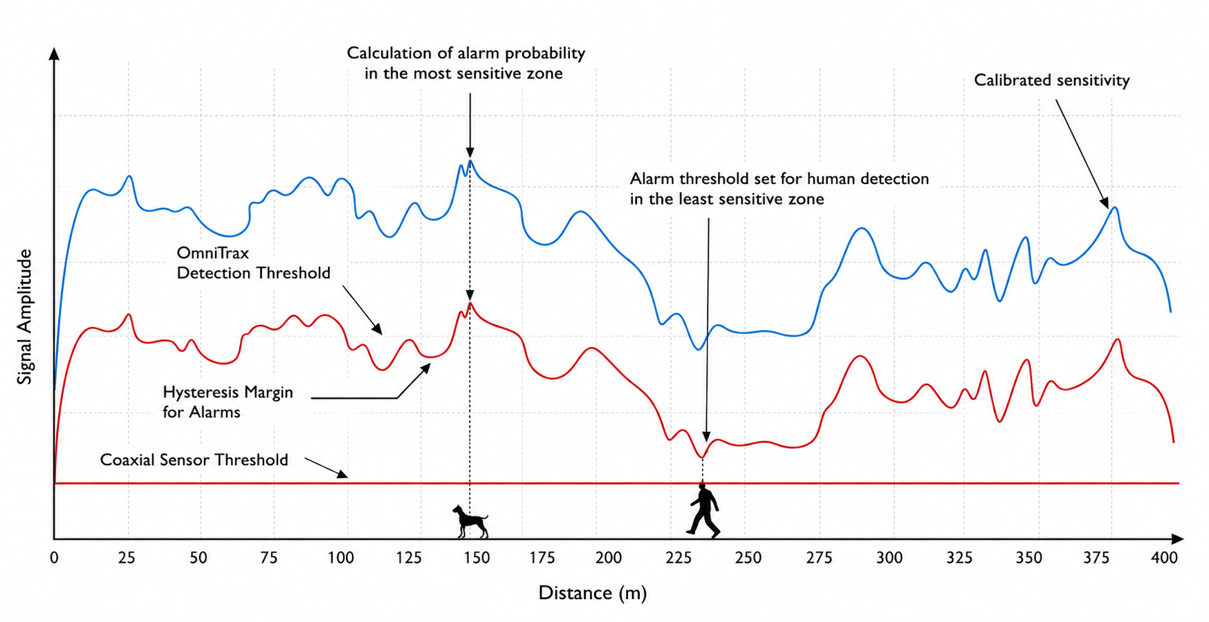
The software automatically records the peak response for each meter of the protected line and creates a sensitivity profile. This profile captures variations caused by installation depth, cable spacing, and soil conductivity, and compensates for these effects.
The benefit of this approach becomes clear when compared with a fixed threshold across the entire cable length. A single threshold would have to be set according to the least sensitive section; otherwise, an intrusion in that area could remain undetected. However, the same threshold would then be too low for the most sensitive sections, making them more likely to generate nuisance alarms. The meter-by-meter sensitivity profile eliminates this compromise.
Sensitivity Balance Control
- Cable margin — 6–24 dB, default 12: provides the global balance between detection probability and nuisance alarm rate.
- Segment correction — ±9.8 dB: enables local sensitivity increase in high-risk areas or reduction in areas with high interference levels.
- Speed filters — 5 settings, independently configurable for slow and fast targets: adjusts the velocity detection window to match threat scenarios.
- STC filter (sensitivity time control — processing time-constant switching) — enabled/disabled, enabled by default: stabilizes response when cables are installed at shallow depth.
The default cable margin is 12 dB, providing a high probability of detection while maintaining a low nuisance alarm rate. The value can be adjusted over time based on accumulated operational data.
Self-Test and Supervision
Supervised items include the sensor cable (open circuits, short circuits, and ground faults), the input section (integrity), the enclosure (tamper switch status), the controller (critical operating parameters), the power supply (power loss and battery status), and the auxiliary inputs (input state and line supervision). The self-test function verifies sensor cable condition and confirms transmitter operation.
The fault relay is configured by default to enter the alarm state when input power is lost. The supervision relay activates on power loss only when the backup battery is missing, not charged, or discharged below the defined threshold — in other words, a healthy backup battery keeps the system in the normal state. The fail-safe operating mode can be configured individually for each of the four relays.
Network-transmitted diagnostics include: enclosure tamper status, program flash memory errors, RAM errors, boot failures, expansion card faults, power supply faults on each bus, battery faults, loss of input power, supervision status for each cable segment, and detected interference.
How to Calculate the System Configuration
The calculation starts with the total perimeter length. The process is as follows:
- Sensor cable length. The usable coverage of a cable kit is approximately 95%: a 400 m kit covers about 380 m of protected perimeter. The required cable length should therefore be calculated with approximately 5% additional allowance above the perimeter length.
- Number of cable kits. Divide the protected perimeter length by the usable coverage length of the selected cable type.
- Number of controllers. Each controller supports two cable kits.
- Power supply. One 48 V power source supports up to five controllers.
- Network and accessories. Install a communication card in each controller, termination loads at the ends of the open perimeter loop, isolators at cable kit junctions, and a surge protection kit for each controller.
Example: 1,500 m perimeter, soil conditions
| Item | Calculation | Result |
|---|---|---|
| Usable OC2 400 m kit length | 400 × 0.95 | ≈ 380 m |
| Required cable kits | 1,500 ÷ 380 = 3.95 | 4 OC2 kits, 400 m each |
| Coverage | 4 × 380 | 1,520 m |
| Controllers | 4 kits ÷ 2 kits per controller | 2 controllers |
| Available alarm zones | 2 × 50 | Up to 100 |
| 48 V power sources | Up to 5 controllers per source | 1 |
| Communication cards | One per controller | 2 |
| Surge protection kits | One per controller | 2 |
| Termination loads | At both ends of the protected line | 2 kits |
The design includes a 20 m coverage reserve and substantial spare alarm zone capacity. Both controllers are powered from a single 48 V source.
When integrating with video surveillance, the available zone capacity enables detailed perimeter segmentation: individual zones can be assigned to camera views, gates, and areas with different risk levels.
Standards Compliance
- Safety — IEC 60950-1, CSA 60950-1-03, SELV, Class 1.
- Radio frequency emissions and susceptibility — CE, FCC (Part 15, Paragraph B), Industry Canada.
- Hazardous substance restrictions — RoHS2.
- Government approval — approved for use by the UK Government.
- Manufacturing — facility certified to ISO 9001:2015.
Summary
OmniTrax is a concealed range-based intrusion detection perimeter system built from a small number of component types: a controller, two types of sensor cable, isolators, termination loads, and a range of expansion cards. A single controller covers up to 800 meters of the protected boundary; longer perimeters are built by grouping controllers.
Three properties define its role in the system architecture.
Concealed perimeter
The detection boundary remains invisible to an intruder, providing no visual reference for planning a crossing attempt while preserving the site’s appearance.
Coordinate instead of zone
Accuracy of ±1 m changes the response model from “a section has triggered” to “a target is located at a specific point”, providing direct integration with video surveillance systems.
Infrastructure cost reduction
The sensor cable simultaneously functions as the sensing element, power line, and data communication line — one installation route replaces three separate infrastructures.
At the same time, this is a system whose performance characteristics are determined together with the site conditions: soil type, installation depth, and cable spacing define the actual detection zone dimensions. The project therefore does not begin with equipment selection — it begins with a site survey, which provides the baseline data for all subsequent calculations.
FortiSec is an engineering partner for perimeter security projects. FortiSec engineers perform site surveys, design zone and controller architectures based on the specific perimeter geometry, verify compatibility with the existing security management system, and support commissioning and system startup. If you are evaluating a buried perimeter detection system for a specific site, send us the perimeter layout and we will prepare a preliminary system configuration calculation.